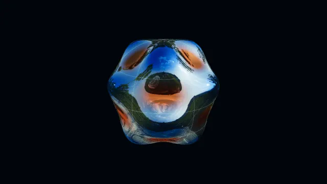
Mathematical reference
- Order zero, radial index two
- Interior radius j₀,₁/j₀,₂ ≈ 0.4357 of the unit disk radius
- Order zero, radial index three
- Interior radii ≈ 0.2779 and 0.6379; these are not equal subdivisions
- Angular factor
- cos(2φ) has four zero rays forming two nodal diameters; its radial factor uses J₂
Lesson transcript
This is the text of the narrated lesson. References to turning, highlighting or changing an object describe the linked interactive lesson; its demonstrations are not embedded in this reading page.
Read a spatial coordinate
Start with the simplest circular drum mode, angular order zero and radial index one. The radial graph runs from the centre at r zero to the rim at r one. Its vertical value records a spatial profile. It is not the history of one point moving up and down in time.
At the centre, J zero of zero equals one. At the rim, the argument is the first positive zero of J zero, approximately two point four zero four eight, so the value is zero. This choice of argument makes the mathematical profile meet a fixed boundary rather than cutting off a nonzero height.
Because angular order is zero, the value does not depend on direction around the centre. Every point at the same radius has the same spatial value. Sweep the radial profile around the centre in your view of the surface: a single curve determines the whole circularly symmetric shape.
Now let the native phase oscillator run. The entire spatial profile is multiplied by one time factor. Every nonzero point passes through zero at certain instants, while the rim remains zero throughout. A momentary flat surface and a permanent node are different mathematical statements.
An interior zero becomes a circle
Select radial index two while keeping angular order zero. The argument now reaches the second positive zero of J zero at the rim, approximately five point five two zero one. The first zero occurs before the rim, so the radial profile changes sign once inside the disk.
To locate that interior zero, solve j zero two times r equals j zero one. The radius is their ratio, about zero point four three five seven. Every direction at that radius gives the same zero, so the graph crossing becomes a complete nodal circle on the drum.
The central region and outer annulus have opposite spatial signs. During oscillation they move in opposite directions, but their common nodal circle does not move. A material reflection can change as the view changes; the calculated zero radius remains a property of the selected function.
At phase zero the whole membrane is flat. The graph still retains the radial spatial profile and its zero crossing. This is a useful test: identify a permanent node from the profile or from its persistence through an oscillation, rather than from one flat frame.
Ratios locate every interior ring
Select radial index three. Its boundary root is approximately eight point six five three seven. Two earlier positive roots now lie inside the argument interval, so the drum has two interior nodal circles. The outer fixed rim is an additional boundary, not one of those interior circles.
Divide the first root by the third to locate the inner ring. The radius is about zero point two seven seven nine. Divide the second root by the third for the next ring, about zero point six three seven nine. These are different spacings, not equal subdivisions of the unit radius.
Watch the same mode oscillate without changing those radii. Three radial sign regions move with alternating signs, separated by two stationary circles. The graph and surface tell the same story: positive and negative intervals along a radius become positive and negative annular regions.
Predict radial index four. It uses the fourth root at the boundary and therefore has three earlier roots inside. Their ratios to that fourth root give three interior circles. The count is easy to predict, while their exact positions require the actual Bessel roots.
An angular factor adds diameters
Change to angular order one and radial index three. The function now multiplies a J one radial factor by cosine phi. One nodal diameter separates opposite angular signs. The radial factor also changes when the order changes, so the old J zero ring radii cannot simply be reused.
At the centre, J one of zero equals zero. That removes any conflict between different angular directions meeting at one point. For every positive integer order, the regular Bessel solution tends to zero at the centre; order zero is the special case that starts at one.
Select angular order two with the same radial index three. Cosine of twice phi has four zero rays around a full turn; opposite rays join into two diameters. The two interior nodal circles remain in number, but their radii now come from zeros of J two.
A radial graph describes a slice at a chosen angular factor. The complete surface multiplies that radial value by the angular value at each point. A zero of either factor makes the product zero, explaining why circles and diameters coexist in the same nodal pattern.
Compare actual rings across radial and angular choices
Return to angular order zero and radial index two. The one interior ring occurs at the first J zero root divided by the second, approximately zero point four three six of the unit radius. It is not halfway to the rim. The graph crossing and the native ring identify the same radial location.
Change to radial index three, still at angular order zero. The first interior ring moves inward to about zero point two seven eight, and a second appears near zero point six three eight. Changing the boundary root rescales every earlier root’s radial position. The original ring is not simply retained while another is inserted.
Approach the outer interior ring of this third mode. The adjacent annuli have opposite spatial signs, separated by a zero at the same radius in every direction. The radial graph records that sign change as a crossing. The full circular node follows because angular order zero contributes no directional variation.
Keep radial index two but change angular order to one. The interior ring now lies at the first J one root divided by the second, approximately zero point five four six. This differs from the J zero ring at the same radial index. Order changes the radial equation as well as adding an angular factor.
At order one, the cosine angular factor vanishes along one diameter. That diameter and the interior circle are simultaneous zeros of the full product. Look across their intersection, then return to the whole disk. Neither a ring count alone nor a diameter count alone describes the complete stationary nodal set.
Keep permanent zeros separate from instantaneous flatness
Select angular order two and radial index two at the positive phase peak. The spatial pattern has one interior circle and two nodal diameters. Its positive and negative regions form alternating sectors on both sides of the circle. These zero locations belong to the spatial function before any time factor is applied.
Set the phase to zero. The entire displayed drum becomes flat, including points whose spatial values are nonzero. The lesson graph retains the spatial profile, so its sign regions and root remain available for comparison. A zero displacement in this single frame is not sufficient evidence that every point is a permanent node.
Set the phase to three pi over two. The time factor is negative one, reversing every nonzero displacement from the positive peak. The nodal circle and diameters remain fixed. Compare the relief from a lower view to see the sign reversal while retaining the rim as a reference plane.
Let the phase vary continuously for the same selected mode. Each nonzero region alternates above and below the reference plane, while the calculated nodes stay at zero. The neighboring regions have opposite spatial signs, so their instantaneous displacements oppose one another. The oscillation changes the time factor without changing the Bessel root or angular order.
Return to a positive peak and reduce amplitude to one quarter. The relief becomes shallower, but the spatial zeros remain the same. Phase and amplitude both scale displacement; changing the mode changes the underlying function. Keep those operations separate as the final chapter compares display scale with the mathematical profile.
Separate mathematical profile from display scale
Reduce display amplitude to one quarter. The rendered relief becomes shallow, but the zeros of the selected mode stay in the same places. The profile graphs use unit-peak normalization so that different modes can be compared; they do not expand and shrink with the surface amplitude slider.
Raise amplitude to three quarters. It is three times the previous display setting. At a fixed point and fixed phase, displacement scales by that same factor. Node locations do not change because multiplying zero by any amplitude still gives zero.
Return to the order-zero third radial mode at the positive phase peak. Reconstruct it from the graph: centre value one, first zero near zero point two seven eight, second near zero point six three eight, and a zero at the rim. Rotating this profile around the centre gives the full spatial pattern.
Choose Interact and select another radial index. Predict the number of interior rings, identify the boundary root, and divide earlier roots by it to locate the rings. Then change angular order separately. This keeps the radial count, actual radii, angular diameters and time phase as distinct quantities.