Reading a Vibrating Surface

What stays still?

Parts of this drum rise while neighboring parts fall. Yet two circles inside the rim remain still. Those circles reveal more about the mode than any single frozen shape. A mode is a spatial pattern multiplied by an oscillation in time. We will separate what belongs to the pattern from what belongs to the moment at which you look.

Freeze the pattern at a positive peak of its time factor. Read the radial graph from center to rim. Its two interior zero crossings become circles when swept around the disk. The outer endpoint is also zero because the rim is fixed. This graph displays the spatial profile, not the up-and-down history of one point. Keeping that distinction prevents a common mistake when comparing a moving surface with a stationary curve.

Separate position from time

Let us read the equation one symbol at a time. The letter u means displacement from the rest surface. The variables r and phi specify a point on the drum: distance from the center and angle around it. The variable t specifies when we look. F is the spatial mode, so F tells us the relative displacement assigned to each position. A controls amplitude. The sine factor tells all those positions how their displacements change together. Multiplication matters here: we first evaluate F at a position, then multiply that number by A and by the sine of the phase. We are not moving the graph sideways across the drum.

For this order-zero mode, the center has spatial value one. Freeze phase at pi over six. The sine of pi over six is one half. With amplitude set to one half, the mathematical displacement at the center is one quarter: one half times one times one half. A position where F equals negative one half would instead have displacement negative one eighth. Both calculations use the same time multiplier. The World applies an additional fixed visual height scale when drawing the surface, so screen pixels are not physical displacement units. The calculation tells us the sign and relative size before that display conversion.

Now phase is pi over two, and the sine factor is one. At the center, displacement is one half rather than one quarter. Every other point has also doubled its displacement relative to the previous frozen state. But a spatial zero remains zero, because zero multiplied by either time factor is still zero. This gives a practical test for a standing mode: compare two nonzero snapshots. If the entire spatial pattern changes by one common multiplier, it can be a single standing mode. If different parts change their relative heights, more than one independently evolving mode is generally involved.

Amplitude changes height, not nodes

Reduce amplitude to one quarter. The relief becomes shallow, but the nodal circles have not moved. Amplitude is a multiplier: it changes the magnitude of displacement, not the radial positions at which the spatial function vanishes. The graph retains its normalized scale so that you can compare the underlying mode independently of the surface display amplitude.

Now amplitude is three quarters, three times the previous setting. The peaks and troughs are more pronounced. Count the circles again: still two inside the rim. Before experimenting, predict which operation could move them. Changing amplitude cannot; selecting a different radial mode generally can. Pause the lesson, try the amplitude slider, then resume to return to this example.

Displacement and velocity are different

A stationary-looking snapshot cannot tell us whether the membrane is moving. Velocity is the time derivative of displacement. Differentiating sine gives cosine, and differentiating its argument supplies omega. The blue graph shows the sine time factor; the orange graph shows the cosine velocity factor after dividing out amplitude, frequency, and the spatial value. At phase zero the blue curve is zero but the orange curve is one. The membrane is passing through its rest surface with its greatest speed at each nonnodal point. Flat therefore does not mean stopped. At permanent nodes the spatial factor is zero, so both displacement and velocity stay zero.

At phase pi over two the roles reverse. The sine is one and the cosine is zero. Displacement is at an extremum, while instantaneous velocity is zero. The membrane is turning around. It will not remain there, because its acceleration points back toward equilibrium. Differentiating once more gives acceleration equal to negative omega squared times displacement. The minus sign expresses the restoring direction. This is why the peak state is a useful starting point for our presets: it describes release from rest, with an initial shape and no initial velocity. The subsequent motion is determined by the wave model.

Predict the next quarter-cycle. Starting at the positive peak, phase increases to pi. Displacement returns to zero, but the velocity factor is now negative one. The drum is crossing its rest surface in the opposite direction from phase zero. Those two flat snapshots look identical, yet their futures differ. This is a basic reason a dynamical state requires both position and velocity. Here the phase control encodes that distinction. Pause, compare phase zero with phase pi, then animate from each state. Look for the direction of the first motion, rather than expecting the two frozen surfaces to distinguish the states.

A zero instant is not a nodal pattern

At phase zero the complete membrane is momentarily flat. Every point has zero displacement at this instant. It would be wrong to call every point a permanent node. A node must remain at zero throughout the oscillation. The radial graph still shows the spatial mode and its two interior roots, even while the time multiplier makes the instantaneous surface flat.

At three pi over two, the time multiplier is negative one. Every raised region from the positive peak is now depressed, and every depressed region is raised. The nodal circles are unchanged. Phase chooses where we are in the oscillation; amplitude chooses its size. Neither parameter selects a new spatial mode.

Read signs and count regions carefully

Return to angular order two and radial index three. The spatial mode is a product of a radial Bessel factor and cosine of twice phi. Along the direction phi equals zero, the cosine is one, so the radial graph directly gives the sign of the mode. Along phi equals pi over two, the cosine is negative one, so the same radial profile is reversed. Along phi equals pi over four, the cosine is zero, so the entire radial ray is a node. The surface is not assembled from separately moving wedges. One product formula assigns a value to every point, and the zero sets of its factors make the boundaries.

Two nodal diameters make four sectors. Two interior nodal circles make three radial bands. In this separated example, each sector meets each band, so there are twelve connected regions away from the nodes. Adjacent regions across a simple nodal line have opposite signs. Do not confuse twelve regions with twelve diameters or twelve circles. The boundaries and the regions they enclose are different counts. At the center several sectors meet at one zero, which does not create an extra band. This exercise connects the graph’s two interior roots, the cosine’s four zero rays, and the visibly repeated patches on the drum.

Now angular order is three and radial index two. Before counting the surface, apply the rule: three diameters give six sectors, and one interior circle gives two radial bands. The answer is again twelve regions. These two modes therefore have the same region count but different geometries. A single visual statistic does not identify a mode. You need both indices, or enough of the nodal structure to recover them. Compare the previous two-circle pattern with this one-circle pattern, and use the order and radial controls to recreate either one. A good description names the actual boundaries, not simply how complicated the image appears.

Read the same idea on two surfaces

Add angular order two. We now have two nodal diameters as well as two interior circles. The diameters divide the drum into four sectors with alternating signs. Watch a full oscillation and distinguish the persistent zero lines from the instant when the entire membrane crosses its rest position. Counting nodes requires watching the pattern, not merely spotting a dark or bright reflection.

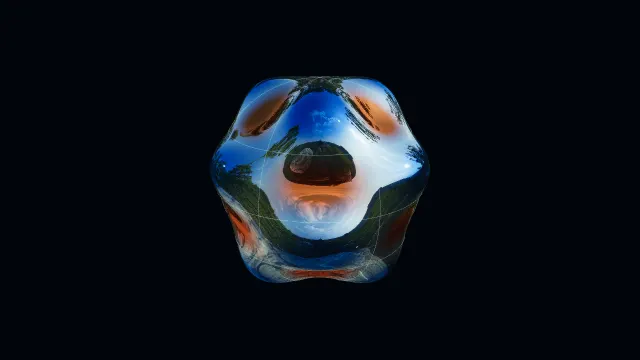
On this undeformed sphere, color displays an angular function of latitude and longitude. Degree six and order three give three interior latitude circles and three nodal great circles. The graphs separate the two factors. Reflections are material lighting; use the signed coloring, graphs, and nodal marks together to read the mathematical function.

Now display that same function as radial deformation. The angular locations of its zeros remain unchanged. You have changed its representation, not its degree or order. Try switching between Sphere and Sculpture yourself. A useful reading routine is to identify the function, locate its zeros, check the amplitude and phase, and only then interpret the apparent motion.

Work a complete reading exercise

Here is a fresh exercise: order zero, radial index four. First predict the interior circle count without inspecting the picture. Radial index four means that the fourth positive Bessel zero reaches the rim, leaving the first three inside. There are therefore three interior nodal circles and four radial sign bands. Because order is zero, there are no nodal diameters. Now check the graph and the surface. Start at the center, follow the bright selected curve, and count only its zero crossings before the right endpoint. The other faint curves are alternative modes in the gallery, not additional roots of this selected function.

Reduce amplitude and freeze at phase zero. The surface becomes flat again, but the three spatial roots still belong to the mode. If someone called this the fundamental because it looked flat, which evidence would correct them? The radial selector still reads four, and the selected graph still has three interior crossings. This is why the lesson keeps the spatial graph separate from the time factor. Each answers a different question. One tells us which mode we selected; the other tells us its instantaneous displacement. Neither should silently replace the other when the membrane happens to cross its rest plane.

Release the same mode and watch those three circles remain fixed. You can now give a complete account: the indices select the spatial function, its roots select the nodal circles, amplitude scales the displacement, and phase selects the instantaneous state. On a spherical harmonic, the same reading method uses latitude and longitude factors instead of radius and disk angle. Before continuing, choose a favorite yourself and explain aloud what stays fixed, what changes with time, and which graph supports each statement. Resume restores the authored example. The goal is to make each visual observation traceable to a particular part of the mathematical model.