One Rule, Many Orbits

The same rule can produce different outcomes

Keep c equal to zero, so every step squares the current complex value. Start at one half. The first image is one quarter, the second is one sixteenth, and the third is one two-hundred-fifty-sixth. The displayed current point approaches zero as the positive values shrink.

Now start at one instead. One squared is one, so the orbit stays at one. This is a fixed point of the same rule. We changed the starting value, not c or the exponent. A fixed point need not be where nearby starting values eventually arrive.

Start slightly beyond it, at one point one. After five squarings, the current value exceeds twenty-one. The trace shows the escape crossing while the readout follows the subsequent values. A small change in the starting value has produced a very different long-term outcome.

Return to one half and the contracting orbit. For a positive real starting value between zero and one, squaring gives a smaller positive value. Repetition drives this particular family toward zero. That exact reasoning is stronger than observing several points that merely seem to stay nearby.

The beginning can differ from the eventual behavior

Begin at i under the same rule. The first image is minus one, because i squared equals minus one. The second image will be positive one. These first points move around the unit circle rather than approaching the origin.

Show the second image, one. It is a fixed point, so every later image is also one. The starting value i and the intermediate value minus one form a transient beginning before the orbit becomes constant.

Advance several more steps. The current value is still one. Overlapping orbit points do not become distinct visible markers just because the step number increases. Read the index together with the position to distinguish time in the sequence from a new location in the plane.

Start directly at minus one. One step now reaches the same fixed point. Different starting values can share eventual behavior while having different transient lengths. We will next compare a repeating cycle with more than one distinct point.

A two-cycle repeats two distinct positions

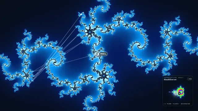
Change the parameter to minus one and start at zero. The first step is zero squared minus one, which gives minus one. The background Julia picture changes because the rule has changed; this is more than selecting another starting point.

Take the second step. Minus one squared minus one equals zero. We have returned exactly to the starting value after two steps, so the same two calculations will repeat forever. This conclusion follows from the rule, not from a numerical resemblance between nearby values.

Advance to the fourth step. The current value is zero again. The least positive repeating period is two, because zero and minus one are distinct. Although the orbit also returns after four steps, four is not its minimum period.

Start instead at one. Its first image is zero, and its second is minus one. It enters the same two-cycle after one transient step. The initial value one belongs to the full orbit but is not one of the two points in its eventual repeating cycle.

Follow a provably growing real trajectory

Keep c equal to minus one and start at two. The first image is three: two squared minus one. This exceeds the radius-two threshold. The native orbit marks where the segment first crosses that circle; the crossing point itself is a drawing aid, not an additional iterate.

Take another step. Three squared minus one gives eight. The current-value readout now says eight, even though the plotted orbit trace is deliberately bounded at its first escape segment. Do not mistake the truncated drawing for a stopped mathematical sequence.

The next image is sixty-three, because eight squared minus one is sixty-three. For these positive real values beyond two, x squared minus one exceeds x by an amount that grows with x. The sequence keeps increasing and cannot settle at a finite limit in this range.

Return to the first crossing. For a quadratic rule with parameter magnitude at most two, an iterate with magnitude strictly greater than two guarantees escape. The strict inequality matters. Crossing the threshold supplies a justified escape certificate; failure to cross in a short computation does not supply the opposite certificate.

Equality at the threshold is not escape

Set c to minus two and start at two. The first image is two squared minus two, which is two again. This orbit lies exactly on the radius-two threshold and is fixed. A test using greater than or equal to two would misclassify it.

Advance to the sixth step. The value is still exactly two in this worked example. The native escape rule uses magnitude strictly greater than the threshold. The threshold is a sufficient test when crossed, not a claim that every point on it escapes.

For contrast, restore c equal to zero while keeping the starting value two. One step now gives four, beyond the threshold. The same starting position can behave differently when the parameter changes. Always name both the rule and its starting value.

Return to the nonescaping fixed example at c equal to minus two. Its proof is the exact identity two squared minus two equals two, repeated indefinitely. We do not need to infer an infinite conclusion from the appearance of a finite trace.

Compare equal magnitudes and different angular histories

Set c to zero and begin at one half on the real axis. After one squaring the magnitude is one quarter, and after two it is one sixteenth. A starting magnitude below one keeps shrinking when squared. The direction of the point is not needed to prove this magnitude statement.

Start instead at one half i, the same distance from the origin. Its first image is negative one quarter, and its second is positive one sixteenth. The angular history differs, but the magnitude sequence is exactly the same. Equal initial magnitudes need not mean equal complex values at every step.

Now use a point of magnitude one: i. Its first image is minus one, its second is one, and later images remain one. This orbit is eventually fixed but the initial point itself is not fixed. The words eventually and initially distinguish two different claims about the same finite trace.

Compare the point one, which is fixed from the first step. Both orbits eventually reach that fixed value, but one has a transient part and the other does not. A finite plot should preserve the starting point and step labels so the common endpoint does not erase those different histories.

Move just outside the unit circle to one point zero one. Six squarings produce a magnitude of one point zero one raised to the sixty-fourth power, still below two. A finite escape test at this stage has not yet crossed the radius-two threshold, even though repeated squaring proves that the orbit will grow without bound.

At the seventh squaring the exponent is one hundred twenty-eight and the magnitude exceeds two. The escape criterion now detects the growth. The change from not-yet-escaped to escaped concerns a finite computational observation; the mathematical orbit did not change its eventual behavior when we increased the number of inspected steps.

Return inside the circle to magnitude one half. Its convergence follows from the exact magnitude rule, while the outside example diverges by the same rule. This is stronger evidence than merely observing several plotted points. Use exact reasoning where available and describe finite numerical evidence honestly where a general proof has not been supplied.

Finite evidence has a clear limit

Choose c equal to one quarter and start at zero. The first image is one quarter; the second is five sixteenths. The current points remain near the real interval from zero to one half. Watch a longer initial part of this orbit next.

Show twelve steps. The values have moved closer to one half without reaching it exactly. In this special real example, the interval from zero to one half is preserved by squaring and adding one quarter. That interval argument proves the orbit stays bounded.

A general finite orbit that has not crossed an escape threshold may escape later. Numerical cycle detection also depends on a tolerance and an observation window. Exact repetition, an invariant interval, and an observed near-return are different kinds of evidence and should not be presented as interchangeable.

Pull back to the complete Julia view. We have compared shrinking trajectories, fixed points, transients, a two-cycle, and certified escape. The next lesson asks how the outcomes for all starting points are organized into a filled Julia set and its boundary.