Complex Numbers as Points and Transformations

A complex value has two coordinates

Begin at the origin of the complex plane. The horizontal coordinate is the real part, and the vertical coordinate is the imaginary part. A value written x plus i y corresponds to the point with coordinates x and y. The symbol i satisfies i squared equals minus one.

Move the starting point to one half on the real axis. Its coordinates are one half and zero, so its imaginary part is zero. Real values occupy this horizontal axis. The highlighted starting point is called z zero; the subscript records the step number, not a multiplication.

Compare minus one half. It lies the same distance from the origin on the opposite side. The sign of a coordinate tells us direction along its axis. It does not make the distance from the origin negative. Both of these starting points have magnitude one half.

Move to i, one unit above the origin. Its real part is zero and its imaginary part is one. We now have a way to represent values that cannot be placed on the real axis alone. The plane gives each complex value a definite position.

Position, distance and direction are different

Choose one plus i. The point lies one unit to the right and one unit above the origin. Its magnitude is the square root of two, from a right triangle with legs one and one. Magnitude is distance from zero, not the sum of the two coordinates.

Compare one minus i. The real coordinate stays one while the imaginary coordinate becomes minus one. Reflection across the real axis changes the sign of the imaginary part. Its magnitude remains the square root of two because the squared coordinate lengths are unchanged.

Compare minus one plus i. This point lies in the upper-left quadrant. It also has magnitude the square root of two, although its direction from the origin differs. Equal magnitudes do not identify equal complex values; position includes direction as well as distance.

Return to one half on the real axis. We will apply a transformation to this starting value. Keep the original point and the next point distinct: a rule maps one value to another, and repeated application creates a sequence of positions called an orbit.

Squaring changes the value

For now the parameter c is zero, so the rule is simply square z. Starting from one half, take one step. The next value is one quarter. The native orbit segment connects the initial point to its image, and the current-value readout identifies z one.

Take another step. One quarter squared is one sixteenth, or zero point zero six two five. We square the current value, not the original starting point again. The second image is closer to zero than either earlier point.

Take a third step. One sixteenth squared is one two-hundred-fifty-sixth, approximately zero point zero zero three nine zero six two five. These positive fractions shrink under squaring because they lie between zero and one. The sequence is approaching zero.

Change the starting value to minus one half and take one step. Its square is positive one quarter. The sign changes because a negative real value multiplied by itself is positive. The two opposite starting points now have the same first image.

Squaring can turn a point

Return to i as the starting value. Its magnitude is one and its direction is a quarter turn counterclockwise from the positive real axis. We will square this complex value using the defining relation i squared equals minus one.

Take one step: i squared is minus one. The image lies on the negative real axis. Complex squaring has changed direction, even though the magnitude remains one. Squaring a complex value is not the same as squaring its two coordinates separately.

Take the next step. Minus one squared is positive one, on the opposite end of the real diameter. A third step leaves one unchanged because one squared equals one. We will display that repeated value next; the sequence has reached a fixed point.

Here is the third step, still at one. A fixed point maps to itself under the rule. The initial point i was not fixed; it reached one after passing through minus one. The early part of an orbit and its eventual behavior need not be the same.

Use both coordinates in the product

Begin again at one plus i with c still zero. Expand its square as one plus two i plus i squared. Since i squared is minus one, the real terms cancel. The result will be two i, not one plus i and not a point with both coordinates squared independently.

Show the first image at two i. It lies two units above the origin. Its magnitude is two, the square of the original magnitude square root of two. Its direction is ninety degrees, twice the original forty-five-degree direction.

Take the next step. Two i squared is four times i squared, or minus four. The orbit moves to the negative real axis and crosses the radius-two escape threshold. The native trace marks that crossing; later numerical values can continue beyond the plotted escape segment.

Return to the first image for comparison. In general, squaring x plus i y gives x squared minus y squared, plus i times two x y. The minus sign and mixed term are essential. Geometrically, squaring squares the magnitude and doubles the angle, measured modulo a full turn.

The parameter adds a translation after squaring

Set the starting value to zero and choose c equal to one half plus one half i. The rule now says square the current value, then add this fixed parameter. The starting point z zero and the parameter c are different inputs, even when one happens to equal the other.

Take the first step. Zero squared is zero, and adding c gives one half plus one half i. The point moves half a unit right and half a unit up. Adding a complex parameter translates the squared result by its real and imaginary components.

Take the second step. One half plus one half i, squared, is one half i. Add the same c again to obtain one half plus i. We have not changed the parameter between steps. Repeated iteration uses the same square-and-add rule on each new current value.

Change c to minus one and return to the starting value zero. The next image is minus one. Changing c changes the rule applied at every step. Changing only z zero would select another orbit of the same rule. A camera move changes neither input.

Separate squaring from addition in one exact example

Start at one half plus one half i with c equal to zero. The point lies in the first quadrant. Its magnitude is the square root of one half and its angle is forty-five degrees. Those two descriptions refer to the same point: one uses coordinates, the other distance and direction.

Apply one squaring. Expanding the product gives one quarter plus one half i plus one quarter i squared. Since i squared is negative one, the real quarter terms cancel. The resulting point is one half i, directly above the origin. Its real coordinate is zero and imaginary coordinate one half.

The magnitude has squared from the square root of one half to one half, and the angle has doubled from forty-five to ninety degrees. Coordinate multiplication and the polar rule agree. Squaring a complex value is not performed by squaring its two coordinates independently; that would omit the cross term and the negative sign.

Keep the same starting point but set c to one quarter minus one half i. After squaring, adding this parameter cancels the imaginary half and adds a real quarter. The first image is therefore one quarter on the real axis. Changing c changed the rule applied to the starting value.

Compare this with moving the starting value to one half on the real axis while restoring c to zero. Its square is also one quarter. The same first image can arise from different combinations of starting point and parameter. A displayed endpoint alone does not tell us which dynamical experiment produced it.

Continue this real-axis example for one more step. One quarter squared is one sixteenth. Each iteration applies the same complete rule to the current value. It does not repeatedly square the original starting point. The orbit index records successive applications, making the dependency between one step and the next explicit.

Return to the original first-quadrant point and its first image. Use Interact to vary the starting point and parameter separately. Predict the real and imaginary components by expanding the square, then compare the native orbit. Maintaining that separation will matter when one plane represents starting points and another represents parameters.

An orbit is a sequence, not a drawn curve

Keep c equal to minus one and take the second step from zero. Minus one squared minus one returns to zero. The first two distinct positions are therefore zero and minus one. The arithmetic now determines what will happen next.

Take the third step and return to minus one. The next step would return to zero again. This is a two-cycle. The lines drawn between the orbit points help us follow their order; the iterates themselves are discrete points, not every point along those connecting segments.

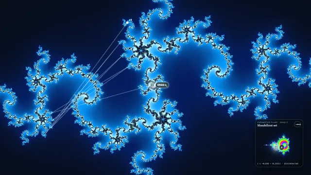
Pull back to the whole Julia view for this fixed parameter. The background summarizes the outcomes of many possible starting points. Our highlighted orbit follows just one of them. The next lessons will connect individual trajectories to this larger picture.

You can now read a complex point, compute its square, add a fixed parameter, and follow the resulting sequence. Keep coordinates, magnitude, starting value, parameter, and camera position separate. Those distinctions will let us compare orbits without confusing a changed rule with a changed view.